Experimenting with PyTorch for Image Approximation using Differentiable Shapes
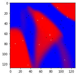
Neural network classifies a random point cloud with random classes(torture mode).
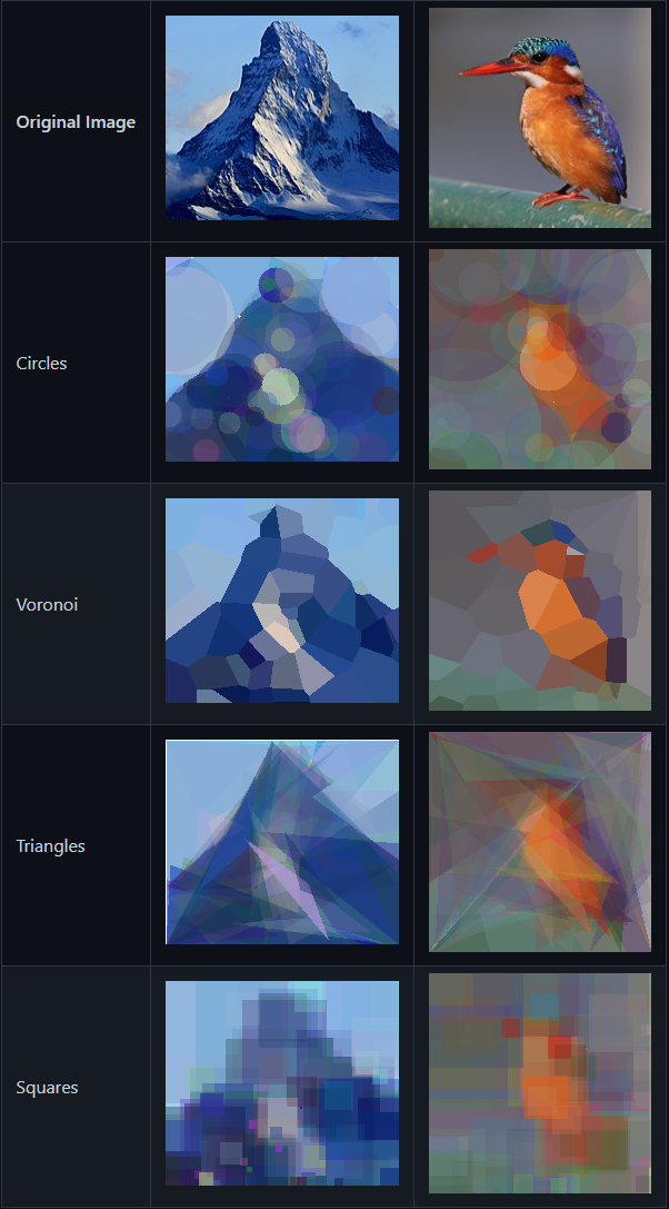
Differentiable shapes approximate an image.
Table of content
Post
Intro
This short post is me sharing an experiment that I find cool. I find it hard to ignore the advances in ML these days. I’d like to learn more and want to do so by starting with something relatable, which is 2d graphics for me. As a beginner in ML, I am embarking on a journey to learn something new and exciting, and to share my observations along the way. I’m not a total noob, but pretty close to it compared to the advances in SOTA at this point. I was attending physics and math classes in the university but due to my obsession with games and programming at the time I didn’t spend much time focusing on the studies, but still some math sinked in.
I’ve discovered this [1] article, it’s interesting but skips some details, the author describes a method to get cool results in a few lines of code and I decided to replicate it and fill in the gaps. In this post, I will be sharing my findings on the experiment of using differentiable primitives for image approximation. I won’t be sticking to the formal definitions and will be trying to explain things in my own wording.
Image Approximation
Image approximation, which is a quite broad topic(JPEG, PNG or any other image compression could be considered an approximation) is a process of finding a method to approximate a signal that is visually similar to the source signal. Compression refers to the process of reducing the size of an image file by altering the data in a way that maintains the quality of the image up to a certain tolerance level. The focus of this post is the use of simple differentiable building blocks in order to approximate an image by minimizing a collective loss, without any practical angle.
Evolutionary Image Approximation
The genetic algorithm is a method for optimizing a problem by iteratively improving a solution through a process that mimics the principles of natural evolution. It involves generating a population of potential solutions, evaluating their quality or “fitness,” and selecting the best ones to serve as the basis for the next generation of solutions. The key aspect of the genetic algorithm that differentiates it from other optimization methods is that it is discrete, meaning that each solution is considered independently and the next iteration of the algorithm involves adding a new entity, rather than continuously updating the current set. This is in contrast to differentiable optimization methods, such as backpropagation, which involve updating the parameters continuously in order to minimize a loss function.
One way to think about the genetic algorithm is as a way to “evolve” a solution to a problem by stochastically navigating a tree of options and selecting the best candidate systems at each step. Each candidate is represented by a “DNA” or a short program that describes it, and the fittest candidates survive to the next iteration, where they are used to generate new variations. I really like the ‘program’ way to think about it. Over time, the algorithm moves towards a better solution by continually selecting the fittest candidates and generating new variations of them. That doesn’t necessarily lead to the globally best solution, but you get something.
One application of the genetic algorithm is in fitting an image. To do this, we would generate a population of potential solutions, each represented by a program that describes how to generate an image. We would then evaluate the quality of each image using an objective function, such as a loss function that measures how well the image matches a target image. Least squared error is quite good. There’s more than that for a perceptual error these days which could lead to a better result. The fittest candidates then would be selected and used to generate new variations, and the process would be repeated. The analogy to biological evolution here is that the candidates represent different species that are evolving over time in response to the demands of their environment, with the fittest ones surviving and reproducing to create the next generation. On a side note, we don’t really know how evolution works but I guess on a high level we do and the name sticks, the same way neural networks are named.
Break through! my simple painting AI can now (try to) paint more complicated shapes. Is genetic algorithm considered AI? I am not sure what is AI these days. pic.twitter.com/sORtiwyTEc
— Shahriar Shahrabi | شهریار شهرابی (@IRCSS) July 6, 2020
Here the author creates images using genetic approximation with different building blocks:
Backpropagation
Backpropagation is an algorithm used to train neural networks, which are machine learning models inspired by the structure and function of the brain(kind of). It is a type of a gradient descent algorithm, which means that it involves adjusting the weights and biases of the network in order to minimize an objective function, such as a loss function that measures the difference between the predicted output of the network and the desired output. A neuron is referred to as a linear layer with a plane equation f(x, p) = tanh(dot(p.n, x - p.bias)). And when you add more neurons to the layer and stack those layers it forms a network.
In order to do the backpropagation we need to analyze the function being optimized f(x, p) in the vicinity of the current weights and biases p in order to determine the direction in which the function is growing the fastest. We then adjust the weights and biases in the opposite direction in order to reduce the value of the objective function. It is important not to overshoot, as the gradient(the rate of change of the function) only provides reliable information about the growth of the function in a small region around the current point. Beyond that vicinity, the gradient may no longer be reliable, and it is possible to miss a local minimum or a saddle point.
One way to think about gradient descent is as a process of path finding in an unfamiliar space. Imagine you are a mosquito searching for a good place to land. You must move around and get a sense of your surroundings in order to locate the source of a smell and determine the direction of the chemical gradient. Similarly, the backpropagation algorithm must adjust the weights and biases of the network in order to find the values that minimize the objective function.
Writing a custom backpropagation framework in C++ is slow and futile. So I’d just go and use a high-level library such as PyTorch these days, which provides automatic gradients and GPU acceleration out of the box. With PyTorch, it is possible to implement and train a neural network in just a few lines of code. You can then save the model and fine tune it to the new input with less computation required. The performance is not ideal sometimes but you can find a way around it and still get results faster than with a custom library.
Here’s an example of a simple neural network in PyTorch that can be trained to classify 2d points.
And the notebook
class SimpleNetwork(nn.Module):
    def __init__(self):
        super().__init__()
        hidden_dimensions = 16
        self.input = nn.Linear(in_features=2, out_features=hidden_dimensions)
        self.hidden_1 = nn.Linear(
            in_features=hidden_dimensions, out_features=hidden_dimensions)
        self.hidden_2 = nn.Linear(
            in_features=hidden_dimensions, out_features=hidden_dimensions)
        self.hidden_3 = nn.Linear(
            in_features=hidden_dimensions, out_features=hidden_dimensions)
        self.output = nn.Linear(in_features=hidden_dimensions, out_features=1)

    def forward(self, xy):
        v = torch.tanh(self.input(xy))
        v = torch.tanh(self.hidden_1(v))
        v = torch.tanh(self.hidden_2(v))
        v = torch.tanh(self.hidden_3(v))
        return torch.tanh(self.output(v))
The result is a function that maps 2d points to the range [0.0 … 1.0] where 0.0 and 1.0 are our classes and everything in-between is up to interpretation based on the tolerated error. I think of hidden layers as a way to figure out a space with more dimensions where the points are linearly separable and then it’s a trivial perceptron fit problem for the output layer.
Differentiable Shapes
Classification is easier to understand in my view, regression has to be more subtle because you need to match the exact function values, not just discrete classes. How do we train a network to place primitives on the 2d image? It feels like a discrete problem. The straight forward answer and the only option covered in this post is to throw more inefficient computation and memory at the problem. In this [1] article the author describes such a method to get cool results in a few lines of code. I’ve implemented basically 1:1 except that I don’t do ordering for simplicity, and make it possible for the color values to go below zero(negative color).
Here’s my notebook
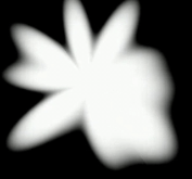
The basic primitive is a ‘fourier shape’ a shape described in polar coordinates as
\[f(\phi, r) = tanh(baseRadius * \sum_{m=1}^{N}(Wsin_{i} * sin(\phi * m) + Wcos_{i} * cos(\phi * m)) - r)\]Which to me looks like a splat.
This shape is defined on the whole 2d plane, you need to evaluate it on the domain in order to compute the final result. It seems localized but the power of the method lies in that it’s not, it’s a continuous function that happen to localize in an area but still has the non zero gradient almost everywhere.
It needs a little bit more than that, an offset, major axes and a scale and then you can scale, rotate and place anywhere on the image.
So by having a list of those and computing an average at the end we can approximate this image:
Into that
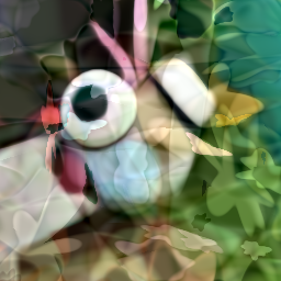
Which is not useful at all but still cool.
Conclusion
This works because the resulting function is differentiable: it’s a sum of functions and each function is a differentiable function. The step forward in accordance with the article [1] is adding another array of f32[num_shapes, isize, isize] or a filter, that acts as a depth buffer really, more or less. It has 1.0 when the shape is visible at the given pixel and 0.0 when it’s not. And we can make the network learn that too. Another step would be adding some sort of texture to the shape so that it looks more like a paint brush.