Thinking about convolutions for graphics
Table of contents
- Table of contents
- Introduction
- Inference oriented point of view
- Pseudocode implementation
- Matrices are graphs
- Low rank operations
- Bonus: my original sketch:
- Links
Introduction
This is a short post about convolutions in the context of graphics processing. While we haven’t switched to vision transformers for everything, CNNs are still the dominant architecture for many tasks and attention is not all we need. In this post I wanted to provide a few sketches that hopefully help understanding and visualizing convolutions in a graphics context.
When introducing convolutions it does often start with something like this:
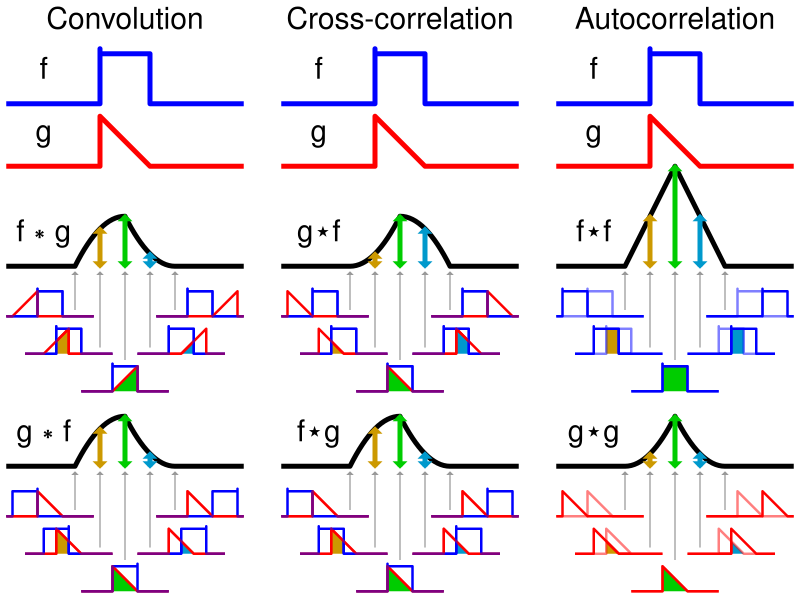
or
Which is fair but from a practical point of view it is not very helpful.
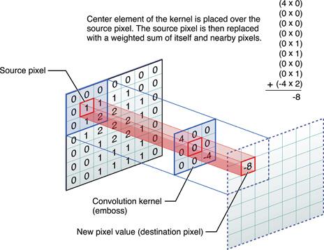
We need to add another dimension which is the feature dimension. In graphics, we usually work with 3D tensors, where the three dimensions correspond to width, height, and feature channels (e.g., RGB). The default layout is referred to as HWC linear layout, which means that we’re linearizing from the last dimension to the first e.g. it will be stored like [R G B R G B ..] in memory for RGB images. When working with ML frameworks the layout is usually BCHW which is batch_size, channels, height, width and in memory it might be stored as an array of 2D ‘grayscale’ single feature slices.
Inference oriented point of view
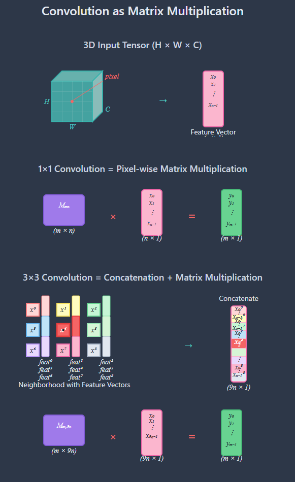
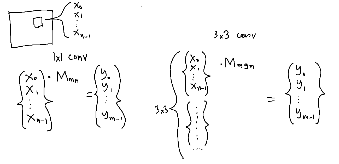
For inference though as we care about the memory hierarchy and hw specific matrix multiplication instructions we want the features to be close to one another and multiple of the number of channels supported by the hardware (4, 8, 16 ..) which also makes thinking about the operations a bit easier, from my point of view.
Everything is a feature vector.
As all we do is just load some vector of values per pixel, multiply it by a matrix and then store that back - pretty straightforward compared to traditional shader workloads. So my point is that this pixel-feature-vector centered point of view makes it easier to think about common operations as we don’t really care that much about the width and heights or batch size during inference, same way we don’t care about the specific pixel locations most of the time for traditional shaders. Also this helps when working with hw matrix multiplication instructions.
Pseudocode implementation
In a naive implementation that would look something like that:
// Compute shader pseudocode
// T - quantized datatype that we use for storage and operations
void Conv1x1(i32x2 tid) {

  vector<T, N> input_features = load<T, N>(input_texture, tid);
  matrix<T, M, N> weights     = load_weights<M, N>(conv1x1_weights);
  vector<f32, M> biases       = load<f32, M>(conv1x1_biases);

  // Matrix multiply
  vector<f32, M> output_features = matmul<T, M, N>(input_features, weights) + biases;

  // Convert back to the quantized domain
  vector<T, M> quantized = quantize<T, f32>(output_features);

  store<T, M>(output_texture, tid, quantized);
}
And 3x3 convolutions would look similar, with just extra concatenation that acts as conditioning of our linear operator on spatially distributed information:
// Compute shader pseudocode
// T - quantized datatype that we use for storage and operations
void Conv3x3(i32x2 tid) {

  vector<T, N * 9> input_features;

  // Load the 3x3 neighborhood of features
  // Or use any other im2col approach
  for (int y = -1; y <= 1; ++y) {
    for (int x = -1; x <= 1; ++x) {
      input_features[(y + 1) * 3 + (x + 1)] = load<T, N>(input_texture, tid + /* offset */ i32x2(x, y));
    }
  }

  matrix<T, M, 9 * N> weights  = load_weights<M, 9 * N>(conv3x3_weights);
  vector<f32, M> biases        = load<f32, M>(conv3x3_biases);

  // Matrix multiply
  vector<f32, M> output_features = matmul<T, M, N>(input_features, weights) + biases;

  // Convert back to the quantized domain
  vector<T, M> quantized = quantize<T, f32>(output_features);

  store<T, M>(output_texture, tid, quantized);
}
And that’s pretty much it. You have your operator implemented. Of course there’s other stuff like padding and stride, dilation but that can be an extension.
# PyTorch convolution
conv3x3 = nn.Conv2d(in_channels=N, out_channels=M, kernel_size=3, stride=1, padding=1)
Matrices are graphs
Another useful perspective is to think of matrices as graphs, where each element is a node and the connections between them represents the strength of the relationship. I recommend reading Matrices and graphs and Matrices and probability graphs.

Low rank operations
It’s often useful as well to have lower rank operations, now that we’re working in the matrix multiplication space. For example, if we have a NxN matrix, the number of flops in a vector-matrix operation is O(N^2). But if we split that matrix into 2 smaller matrices that map half of the input features to another half of the output features, we’ll get (N / 2)^2 * 2 which is 1/2 the original cost. Not hard to notice this has some nice properties, but the downside of this is that during training the disjoint feature groups don’t talk to one another; luckily, we can solve that by adding another MxN matrix multiply after that to combine the features which still could be less than the original cost.
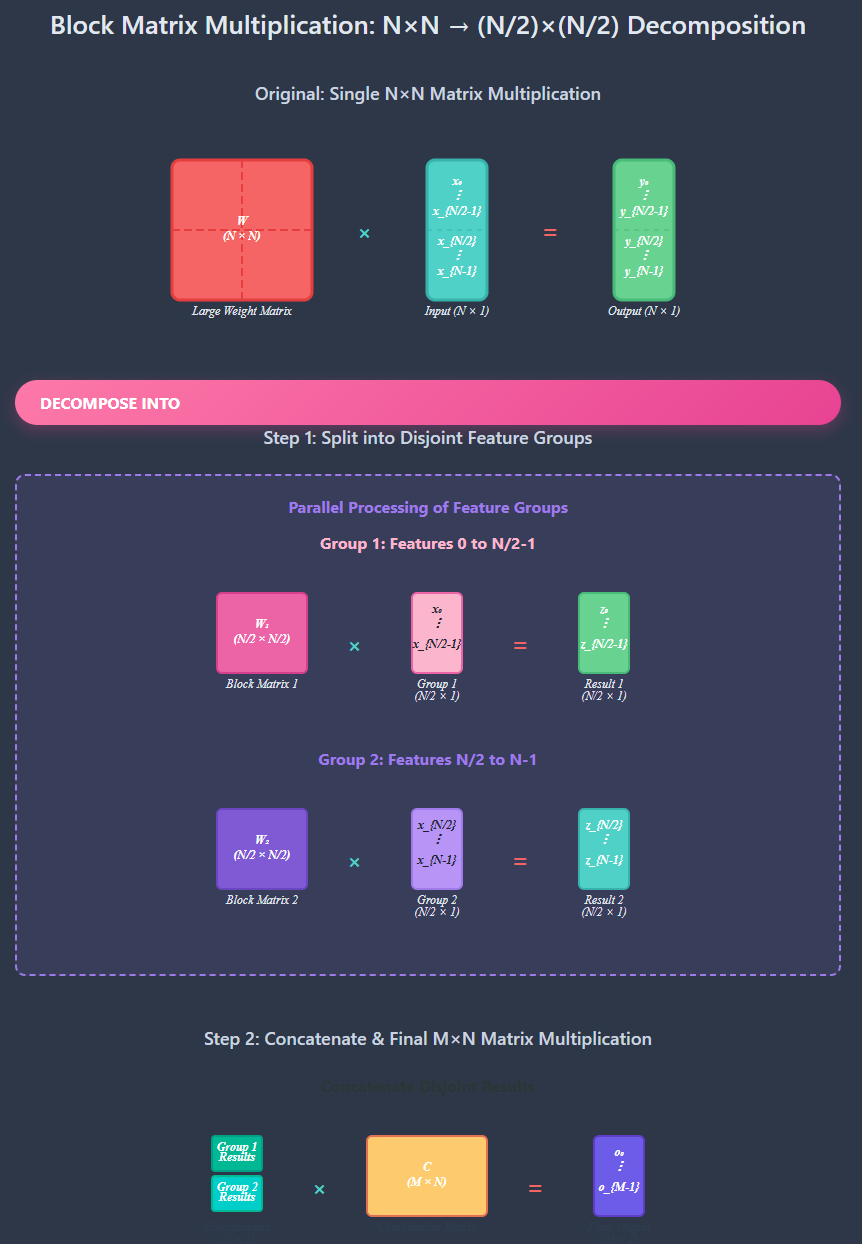
And thinking about the feature vector as a group of features multiple of fixed hw specific matrix size will help you cutting down GOPs and design better operators/fused block.
Bonus: my original sketch:
I ran this through Claude to generate the nice diagrams.
Links
[2]Using the Matrix Cores of AMD RDNA 4 architecture GPUs
[4]Matrices and probability graphs
| Thanks to Nadav Geva for reviewing the draft. |