Table of contents

• Table of contents
• Introduction
• Generic Computation
  • Matrix multiplication - the building block for the era of GPUs
• DAG
• Dynamic graph building
• Parameter Update
• Chain rule
• Auto Grad
• Toy AutoGrad Implementation
• Gradient Noise
• Loss function
• Regularization
• Skip connections
• Detach
• Gradient reset
• Example
• Key takeaways
• Links

Introduction

In this post, I want to share some thoughts on differentiable compute from a practical perspective. It’s a bit unstructured and doesn’t have a story, but I might be updating it over time with new notes.

The goal of this post is to not go into the mathematical details and fundamentals of anything, rather the goal is to hop on the broad set of tools and concepts from a practical perspective and accumulate notes for myself. Pytorch will be primarily focused on.

Generic Computation

There’s many ways to describe a computation but for this post we’ll focus on a process of transforming inputs into outputs through a series of applications of elementary operations or rules that build the result from the inputs. The basic building blocks of computation in ML are operations like addition, multiplication, and more complex functions that can be composed together. In the context of ML for graphics we usually jump straight into convolutions which are matrix multiplications, which are scalar multiplications with additions. I’d say that complexity of ML doesn’t lie in its compute because usually really basic operations are used, rather the complexity is in getting that compute to produce a useful result. It is also somewhat confusing after analyzing the models that stacking simple compute outperforms analytical solutions in both quality and speed, in many empirical cases.

Getting back to matrices, the best way to imagine a matrix-matrix multiplication is via a cube where each cell c_ijk in a cube is a multiplication of elements on its sides A_ik and B_kj, and every element in the result C_ij matrix(third cube side) is a sum reduction(accumulation) along the k axis. You can build a mat mul with just an expand(), element wise multiply and reduce(dim=k). Expand effectively is a way to broadcast values along a new dimension. So we first expand both matrices to have the same 3D dimensions, element wise multiply and then reduce the K dimension.

Source

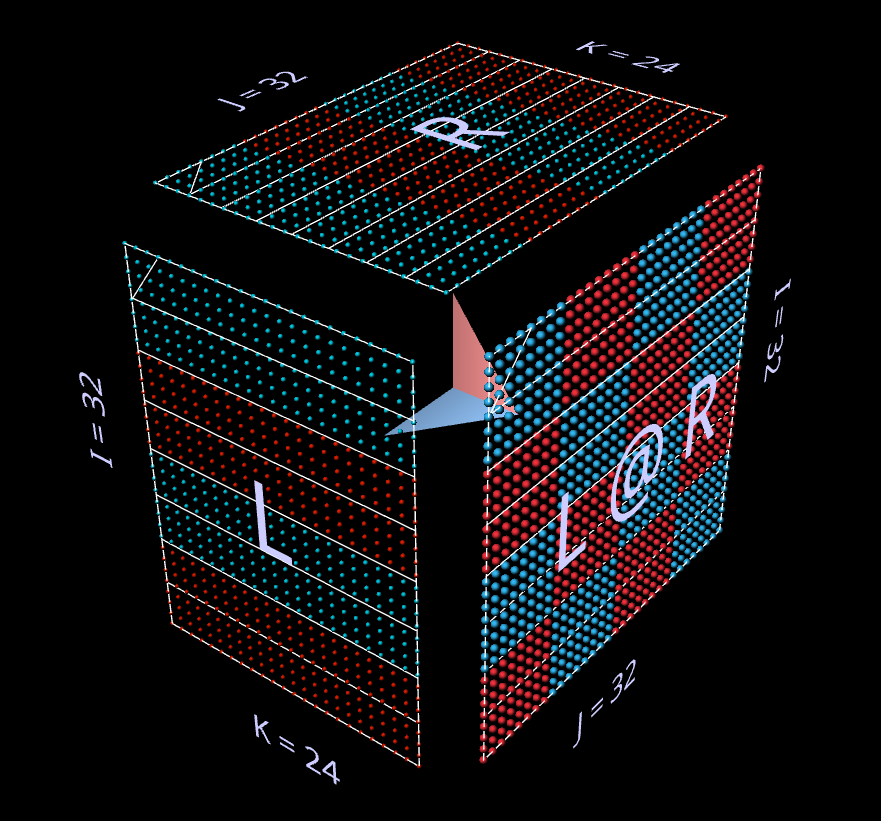
Once you have a grasp on matrix multiplication, you can build most ML models. Matrix expresses a linear fully connected pairwise relationship between an input stack of nodes and an output stack of nodes, that’s generic enough to cover most use cases. Convolutions can be represented as a big matrix multiplication in theory, in practice they are vector-matrix multiplication, but what you can do is to stack/batch the input feature vectors to comprise a matrix and then you’re back to a matrix-matrix multiplication. As long as you have a dot product somewhere you can probably map that to a matrix-matrix multiplication problem.

Matrix multiplication - the building block for the era of GPUs

Something useful to consider is that the memory footprint of a NxN matrix is O(N^2) but the compute required to multiply that matrix is O(N^3). That means that there’s N expressions after the cube expansion for each element in memory, before reduce and if we don’t have to spill to memory and keep everything local it maps pretty well to modern GPU architectures that have orders of magnitude more FLOPS than memory bandwidth. In other words having a large FLOP/byte is what makes the matrix multiplications map well to the hardware, in theory.

The other concept to understand is the reducibility of a series of matrix operations into a single matrix multiplication. This is important for designing the models. There’s sometimes cases when you still want to keep some matrices in a redundant expression but usually you don’t. Also when doing low rank approximations you still keep chains of matmuls. Any scalar, vector or matrix multiplication can be merged as a single matrix multiplication if you reshape the tensors appropriately. What happens then when we want to build a non-linear transformation is that we just apply a non-linear function in-between the matrix multiplications - that way it doesn’t reduce to a single matrix multiplication.

DAG

Directed Acyclic Graph (DAG) is a directed graph with no cycles. Sort of a tree but each node can have more than one parent. In the context of compute graphs, this means that the flow of data and operations moves in one direction, from inputs to outputs, without any causation feedback loops. There’s loops, conditions and jumps in a generic compute graph. Loops are a way to unroll the computation or condition a computation, as the time passes but it doesn’t inverse the causation. In ML compute graphs we usually don’t have loops and jumps or conditions so no need to worry about it at all. We have lerps and when(b, x, y) but that could be rewritten into just lerps. There’s ways things are optimized but effectively you can think of it as if everythinng is computed in an ML compute graph during forward pass, thus we arrive at DAGs. When there’s a loop in the python code what happens is that the compute graph is being built dynamically and all it does is just instantiates a new node in the graph.

Dynamic graph building

Things like:

x = torch.Tensor([1.0], requires_grad=True)

if cond:
    y = x * 2
else:
    y = x * 3

Dynamically builds 2 different compute graphs depending on the condition.

Whereas something like this:

x = torch.Tensor([1.0], requires_grad=True)
y = torch.where(cond, x * 2, x * 3)

Builds a single compute graph with a selector node.

Similarly with the loop:

x = torch.Tensor([1.0], requires_grad=True)
for i in range(5):
    x = x * 2

y = x

Python interpreter executes the loop and appends a new node to the dynamic compute graph for each iteration and x after each iteration points to a new node.

Parameter Update

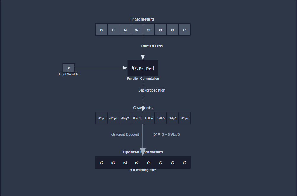
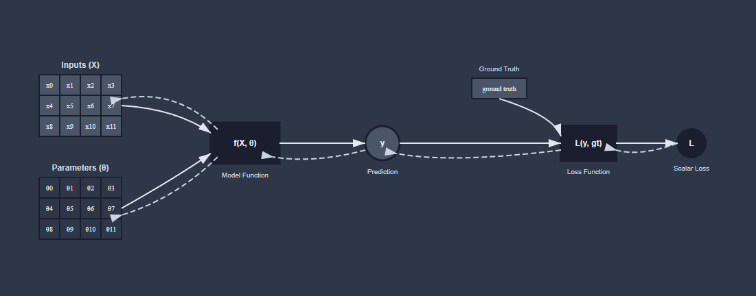
Jumping a bit forward, we perform training by computing the gradients by applying the chain rule through the graph and then in order to minimize our scalar final output we subtract the gradient of the loss function with respect to that node at the terminator nodes(learnable parameters) multiplied by a learning rate, this effectively pushes the parameter vector into the direction of steepest descent given that the function is differentiable and well behaved, and the learning rate is small enough. If we want to optimize for an ensemble of losses, we just add them together or we can run backpropagation multiple times to accumulate the gradients.

The formulas and the expansions of the partial derivative for a parameter are assuming that the other parameters and inputs are constant. This is a linear assumption and that has its limitations, as in reality all parameters are interdependent and the learning rate is not infinitesimal, that’s why we need to be careful selecting the hyperparameters and it takes many learning epochs for all the parameters to adjust to the changes in other parameters.

Usually optimizers like AdamW also track the mean and variance of the gradient to adaptively adjust the learning rate. Other more sophisticated optimizers may use curvature estimates to further improve convergence. But in the crux basic linear gradient descent is all about following the slope.

As you will see the gradients flows into each node, including the inputs. In some applications like neural radiance cache or NeRFs, this can enable pushing the gradients into a fixed grid that helps the encoder.

The way I like to think about the optimization process is that we have a scalar function \(f(x, p_0, p_1, ... p_{n-1})\) Where p is the learnable parameters. Doesn’t matter if we have a single parameter or a matrix or any tensor, it all could be linearized into a vector of scalar values. And that makes it easier to design the optimizer to handle a generic case.

For AdamW we keep exponential moving averages of the gradients and the squared gradients, which we later use to compute the second moment. The intuition here is that high variance in the gradients can indicate areas where the loss landscape is more complex and may require more careful optimization. Coupled with the gradient passing through the temporal low pass filter, this can help stabilize the training process.

How do we get the gradients?

Chain rule

What we’re looking for concretely is a vector of gradients with a scalar gradient value for each parameter p_i:

Before moving forward we need to understand the chain rule. The main idea behind backpropagation is to compute the gradient of a scalar function with respect to its inputs by applying the chain rule of calculus. The chain rule allows us to break down complex functions into simpler components, making it easier to compute gradients by iterating through the compute graph.

Terminator:

If y doesn’t depend on x:

Basically we recursively expand the expressions and apply the derivative and the chain rule at each step starting at L(x, p_0, p_1 …). So as long as what we have is compositions of differentiable functions, we can apply the chain rule at each step. For example, here’s how the derivative rule works for addition and multiplication:

Ok so symbolically for each parameter we just apply the rules at each expression and get down to the target parameters - how does it work in practice?

Auto Grad

Given the chain rule:

y(x) could be any subgraph of the compute graph as long as z(x) = f(y(x)). So we have effectively a way to split the problem in half. In a DAG terminology we have y dominating z on any path to x.

Given that we have a system to build the compute graph. When all the nodes are differentiable, we can apply simple automatic differentiation rules recursively to the compute graph at each node to compute the full gradients automatically.

Given an expression:

We expand every operator to be binary/unary into a list of simple expressions:

And then this could be represented as a compute graph:

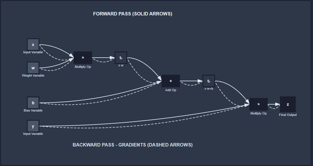
As long as it’s comprised of differentiable operations, we can compute gradients with respect to any input variable and optimize for parameters using backpropagation. I recommend watching Andrej Karpathy for a deeper understanding of these concepts.

It is also preferable to accumulate the gradients for many parameters at the same time at any node before continuing further. It is important for performance, if we, say, have a matrix multiplication we don’t want to follow the nodes depth first, rather we want to compute the gradients for all the input nodes using accelerated matrix multiplies.

Example snippet from TinyGrad:

(UPat(Ops.ADD), lambda ctx: (ctx, ctx)),
...
(UPat(Ops.MUL, name="ret"), lambda ctx, ret: (ret.src[1]*ctx, ret.src[0]*ctx)),

The job for auto grad is to define a rule for each node that specifies how to compute gradients for its inputs, and increment them iteratively. After that the recursive chain rule comes into play. ctx - is the gradient accumulator, ret - is the input values of the node. The system doesn’t compute the complete gradient at each node like we’d do symbolically, rather it increments the gradients as we go.

Toy AutoGrad Implementation

Now lets build a simple AutoGrad system from first principles.

import math
import random

# Compute graph basic building block
class AutoGradNode:
    def __init__(self):
        # scalar valued gradient accumulator for the final dL/dp
        self.grad = 0.0
        # dependencies for causation sort
        self.dependencies = []

    def zero_grad(self):
        self.grad = 0.0

    # Overload operators to build the computation graph
    def __add__(self, other): return Add(self, other)
    def __mul__(self, other): return Mul(self, other)
    def __sub__(self, other): return Sub(self, other)

    # Get a topologically sorted list of dependencies
    # starts from the leaf nodes and terminates at the root
    def get_topo_sorted_list_of_deps(self):
        visited = set()
        topo_order = []

        def dfs(node): # depth-first search
            if node in visited:
                return
            visited.add(node)
            for dep in node.dependencies:
                dfs(dep)
            topo_order.append(node)

        dfs(self)

        return topo_order

    def get_pretty_name(self): return self.__class__.__name__

    # Pretty print the computation graph in DOT format
    def pretty_print_dot_graph(self):
        topo_order = self.get_topo_sorted_list_of_deps()
        _str = ""
        _str += "digraph G {\n"
        for node in topo_order:
            _str += f"    {id(node)} [label=\"{node.get_pretty_name()}\"];\n"
            for dep in node.dependencies:
                _str += f"    {id(node)} -> {id(dep)};\n"
        _str += "}"
        return _str
    
    def backward(self):
        topo_order = self.get_topo_sorted_list_of_deps()

        for node in topo_order:
            node.zero_grad() # we don't want to accumulate gradients

        self.grad = 1.0 # seed the gradient at the output node

        # Reverse the topological order for backpropagation to start from the output
        for node in reversed(topo_order):
            # from the tip of the  graph down to leaf learnable parameters
            # Distribute gradients
            node._backward()

    # The job of this method is to propagate gradients backward through the network
    def _backward(self):
        assert False, "Not implemented in base class"

    # Materialize the numerical value at the node
    # i.e. Evaluate the computation graph
    def materialize(self):
        assert False, "Not implemented in base class"

# Any value that is not learnable
class Variable(AutoGradNode):
    def __init__(self, value, name=None):
        super().__init__()
        self.value = value
        self.name = name

    def get_pretty_name(self):
        if self.name:
            return f"Variable({self.name})"
        else:
            return str(self.value)

    def materialize(self): return self.value

    def _backward(self):
        pass

Constant = Variable

# Learnable parameter with initial random value 0..1
class LearnableParameter(AutoGradNode):
    def __init__(self):
        super().__init__()
        self.value = random.random()

    def get_pretty_name(self):
        return f"LearnableParameter({round(self.value, 2)})"

    def materialize(self): return self.value

    def _backward(self):
        pass

class Abs(AutoGradNode):
    def __init__(self, a):
        super().__init__()
        self.a = a
        self.dependencies = [a]

    def materialize(self): return abs(self.a.materialize())

    def _backward(self):
        self.a.grad += self.grad * (1.0 if self.a.materialize() > 0 else -1.0)

class Square(AutoGradNode):
    def __init__(self, a):
        super().__init__()
        self.a = a
        self.dependencies = [a]

    def materialize(self): return self.a.materialize() ** 2

    def _backward(self):
        self.a.grad += self.grad * 2.0 * self.a.materialize()

class Sub(AutoGradNode):
    def __init__(self, a, b):
        super().__init__()
        self.a = a
        self.b = b
        self.dependencies = [a, b]

    def materialize(self): return self.a.materialize() - self.b.materialize()

    def _backward(self):
        self.a.grad += self.grad
        self.b.grad -= self.grad

class Add(AutoGradNode):
    def __init__(self, a, b):
        super().__init__()
        self.a = a
        self.b = b
        self.dependencies = [a, b]

    def materialize(self): return self.a.materialize() + self.b.materialize()

    def _backward(self):
        self.a.grad += self.grad
        self.b.grad += self.grad

class Mul(AutoGradNode):
    def __init__(self, a, b):
        super().__init__()
        self.a = a
        self.b = b
        self.dependencies = [a, b]

    def materialize(self): return self.a.materialize() * self.b.materialize()

    def _backward(self):
        self.a.grad += self.grad * self.b.materialize()
        self.b.grad += self.grad * self.a.materialize()

a = LearnableParameter()
b = LearnableParameter()

for epoch in range(3000):

    x = Variable(random.random(), name="x")
    z = x * x * a + b
    loss = Square(z - (x * x * Constant(1.777) + Constant(1.55))) # L2 loss to Ax^2+B

    print(f"Epoch {epoch}: loss = {loss.materialize()}; a = {a.materialize()}, b = {b.materialize()}")
    # Backward pass
    # Gradient reset happens internally in the backward pass
    loss.backward()

    # Update parameters
    learning_rate = 0.01333

    for node in [a, b]:
        # print(f"grad = {node.grad}")
        node.value -= learning_rate * node.grad

with open(".tmp/graph.dot", "w") as f:
    f.write(loss.pretty_print_dot_graph())

# Output:
# Epoch 2999: loss = 1.0971718506497338e-07; a = 1.7761125496912944, b = 1.5503818948331147
# Target: 1.777, 1.55

We get this dotgraph at .tmp/graph.dot:

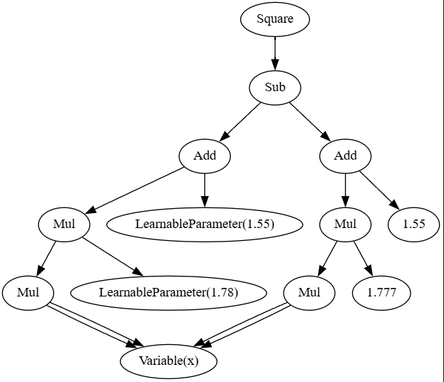
Important takeaway here is that the gradient distribution is a local operator and it’s useful to think that way: addition just passes the gradients to both terms, while multiplication scales the gradients by the value of the other term. We’re sort of solving the inverse problem, instead of revolving around the parameters in a depth first fashion, like we would do symbolically, we recurse into nodes and iteratively accumulate gradients for all the avaliable input nodes at the same time.

On a side note, the auto grad system needs to keep alive most of the time all the intermediate values which expands the memory usage and needs to be taken into account during training to maximize the VRAM utilization. Some functions like ReLU don’t need to store the inputs - the sign is enough for the gradient computation.

Gradient Noise

The gradient is a random variable because our training batch is comprised of a finite number of samples, each with their own noise and variability. This means that the gradient can fluctuate significantly from batch to batch, and it’s crucial for the optimizer to account for this uncertainty. It’s usually the case that it’s not certain that increasing the batch size always helps, the relationship between batch size and the optimization horizon is complex and context-dependent.

Loss function

The loss function is a critical component of the optimization process, as it quantifies the difference between the predicted output and the ground truth in a supervised learning context. The choice of a loss function can significantly impact the training dynamics and the quality of the learned model. Common loss functions include mean squared error for regression tasks and cross-entropy loss for classification tasks.

So far we’ve been discussing backpropagation and its role in computing gradients for optimization. Backpropagation relies on the chain rule of calculus to compute gradients through the computational graph, allowing us to update model parameters in the direction of steepest descent. But that only works when the function is scalar-valued. This is not usually the case so we need the loss function to terminate our compute graph and produce a scalar output that we can minimize for and push the gradients to the learnable parameters.

The loss function not only provides a scalar output for optimization but also serves as a guide for the learning process. By shaping the loss landscape, it influences how gradients are propagated back through the network, ultimately affecting the learned representations and model performance.

Often the case that ground truth is not perfectly achievable or it has inherent error, and the loss function must be robust to these factors as well as making sure that the tradeoff that the model achieves with respect to its limited capacity is appropriate for the target task. This is where data augmentation, regularization, robust loss functions and other techniques to smoothen the loss landscape come into play to kick out the model from trivial overfitting or just not generalizing enough.

Regularization

For image tasks common techniques for data augmentation include random cropping, flipping, rotation, shearing, scaling, mixups and color jittering. These techniques help to create a more diverse training dataset, making the model more resilient to variations in the input data.

Common regularization techniques include L1 and L2 regularization, dropout.

We effectively add the sum of magnitudes of the parameters to the loss function, which is not what happens practically for AdamW, for example, when the weight decay is decoupled from the main loss function gradients.

L2 regularization, in particular, minimizes surprise assuming the weights have a Gaussian distribution prior and reduces the amount of information in the parameters(corresponds to maximizing the posterior under a zero-mean Gaussian prior on weights/MAP), it pushes the weights to be smaller and don’t have high variance.

L1 encourages sparsity in the model weights, promoting simpler models because the gradient is constant until the weight reaches zero, so for weak weights it can effectively remove them from the model.

Dropout randomly drops units from the network during training, forcing the model to learn more robust features in the multi-dimensional space that are less reliant on specific activations. Dropout could also be applied to the input features as well.

Skip connections

Skip connection is nothing special, it’s just a way to formulate your transformation in such a way that allows the gradients to flow more easily through the network by creating shortcuts between transformations.

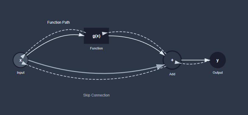
This could be thought of as g(x) computing the delta to the input, rather than computing a whole new function, that somewhat makes it easier for the network to learn specific things that would otherwise require it to first learn the identity.

The effective gradient at x will be such(L is the loss function):

So g(x) acts as a delta to the identity gradient.

During backpropagation we first add f gradients(dL/df) to x, then continue recursing into g(x):

x.grad += f.grad

# g.backprop()

...

# after recursing into g(x) at some point

x.grad += f.grad * grad_from_g # 'f.grad *' is not explicit usually and is just factored in the accumulator

Again, x could be anything, it could be a hidden state, an input feature, or even the output of another layer. The beauty of backpropagation and the chain rule is that it solves the problem one node at a time.

Modern architectures often use skip connections extensively, particularly in deep networks like ResNets. There’s more variations of different skips like SwiGLU used in modern LLMs [3]:

What it does is makes it easier for the network to learn quadratic relationships x * y in just one layer [4] whereas with a normal MLP+relu you’d need 3 layers to learn that relationship.

Detach

Detaching a tensor from the computation graph is useful when you want to stop tracking gradients for a particular tensor. This can be done using the .detach() method or torch.no_grad(). This will create a new tensor that shares the same data but will not propagate gradients and will act as a constant value during backpropagation.

x = y.detach() # Detach y from the computation graph

with torch.no_grad():
    # Perform operations without tracking gradients

One useful application of that is when combining with non-differentiable operations:

x = x + (f(x) - x).detach() # Combine with non-differentiable operation like quantization or clamping

This will pass the gradients through the detached tensor by combining it with the original tensor.

Gradient reset

By default pytorch .backward() accumulates gradients and releases the computation graph to save memory, so you need to zero them out manually after each optimization step.

optimizer.zero_grad()

This is important because if you don’t flush the gradients, they will accumulate over multiple optimization steps, leading to incorrect updates.

That could be a good thing as well, if you want to minimize memory usage you could try to accumulate gradients multiple times for different loss functions calling loss[i].backward(). On each iteration, in theory, it will only allocate the temporary tensors needed for a given loss function, but that depends.

Example

import torch
import torch.nn as nn
import torch.optim as optim

class SimpleNet(nn.Module):
    def __init__(self, input_size, hidden_size, output_size):
        super().__init__()
        self.layer1      = nn.Linear(input_size, hidden_size) # matrix multiplication layer
        self.layer2      = nn.Linear(hidden_size, output_size)
        # inplace=True will modify the input tensor directly(unsafe if the input is shared)
        self.activation  = nn.ReLU(inplace=True)
        self.dropout     = nn.Dropout(0.05) # dropout activations with 5% probability

    def forward(self, x):
        # This builds the compute graph dynamically
        h = self.activation(self.layer1(x))  # Non-linearity breaks matrix chain
        h = self.dropout(h)  # Apply dropout
        y = self.layer2(h) + x # skip connection
        # Quantize symmetrically to int8 using scale 1.0 / 127.0
        y_quantized = (y.detach() * 127.0).round().clamp(-128.0, 127.0) / 127.0
        return y + (y_quantized - y).detach()

# Training loop demonstrating the concepts
model     = SimpleNet(10, 5, 1)
optimizer = optim.AdamW(model.parameters(), lr=0.001, weight_decay=0.01) # learning rate and weight decay
criterion = nn.MSELoss() # mean squared error loss

for epoch in range(100):
    # Forward pass - builds compute graph
    outputs = model(inputs)
    loss = criterion(outputs, targets)  # Scalar terminator
    
    # Backward pass - applies chain rule through graph
    optimizer.zero_grad()  # Reset gradients
    loss.backward()        # Compute gradients
    optimizer.step()       # Update parameters

Key takeaways

1. The computation graph is built dynamically during the forward pass, allowing for flexible model architectures.
2. Autograd in PyTorch automatically computes gradients for all operations on tensors with requires_grad=True, simplifying the backpropagation process.
3. Regularization techniques like dropout can help prevent overfitting by randomly deactivating neurons during training.
4. Weight decay is a regularization technique that adds a penalty on the size of the weights to the loss function, helping to prevent overfitting.
5. Loss function should be selected based on the specific task, data characteristics and trade-offs for a given problem.
6. Detaching tensors can help manage gradient flow, especially when combining with non-differentiable operations.
7. It’s crucial to reset gradients after each optimization step to prevent incorrect updates.

Links

[1]Andrej Karpathy: The spelled-out intro to neural networks and backpropagation: building micrograd

[2]TinyGrad: A minimalistic deep learning library

[3]SwiGLU: A New Activation Function for Neural Networks

[4]What is SwiGLU? A full bottom-up explanation of what’s it and why every new LLM uses it

[5]All the Activation Functions

[6]Understanding PyTorch AutoGrad: A Complete Guide for Deep Learning Practitioners

[7]What Does the backward() Function do?